Key Classification Concepts
Please take a look at these videos where you learn basic steps in eCognition:
Getting Started 1 of 4: Create a project
Getting Started 2 of 4: First dynamic classification
Getting Started 3 of 4: Improve your objects
Getting Started 4 of 4: Export your results
Assigning Classes
When editing processes, you can use the following algorithms to classify image objects:
- Assign Class assigns a class to an image object with certain features, using a threshold value
- Classification uses the class description to assign a class
- Hierarchical Classification uses the class description and the hierarchical structure of classes
- Advanced Classification Algorithms are designed to perform a specific classification task, such as finding minimum or maximum values of functions, or identifying connections between objects.
Class Descriptions and Hierarchies
You will already have a little familiarity with class descriptions and hierarchies from the basic tutorial, where you manually assigned classes to the image objects derived from segmentation..
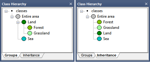
There are two views in the Class Hierarchy window, which can be selected by clicking the tabs at the bottom of the window:
- Groups view allows you to assign a logical classification structure to your classes. In the figure below, a geographical view has been subdivided into land and sea; the land area is further subdivided into forest and grassland. Changing the organization of your classes will not affect other functions
- Inheritance view allows class descriptions to be passed down from parent to child classes.
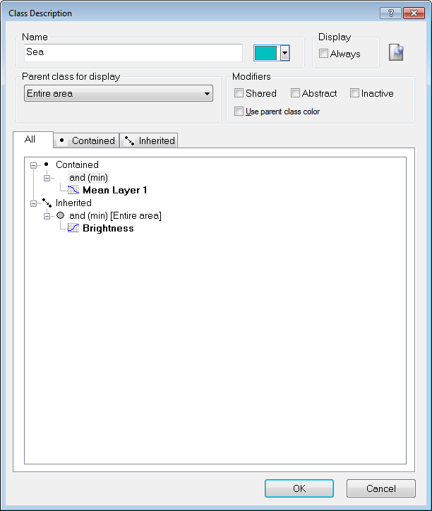
Double-clicking a class in either view will launch the Class Description dialog box. The Class Description box allows you to change the name of the class and the color assigned to it, as well as an option to insert a comment. Additional features are:
- Select Parent Class for Display, which allows you to select any available parent classes in the hierarchy
- Display Always, which enables the display of the class (for example, after export) even if it has not been used to classify objects
- The modifier functions are:
- Shared: This locks a class to prevent it from being changed. Shared image objects can be shared among several rule sets
- Abstract: Abstract classes do not apply directly to image objects, but only inherit or pass on their descriptions to child classes (in the Class Hierarchy window they are signified by a gray ring around the class color
- Inactive classes are ignored in the classification process (in the Class Hierarchy window they are denoted by square brackets)
- Use Parent Class Color activates color inheritance for class groups; in other words, the color of a child class will be based on the color of its parent. When this box is selected, clicking on the color picker launches the Edit Color Brightness dialog box, where you can vary the brightness of the child class color using a slider.
Creating and Editing a Class
There are two ways of creating and defining classes; directly in the Class Hierarchy window, or from processes in the Process Tree window.
Creating a Class in the Class Hierarchy Window
To create a new class, right-click in the Class Hierarchy window and select Insert Class. The Class Description dialog box will appear.
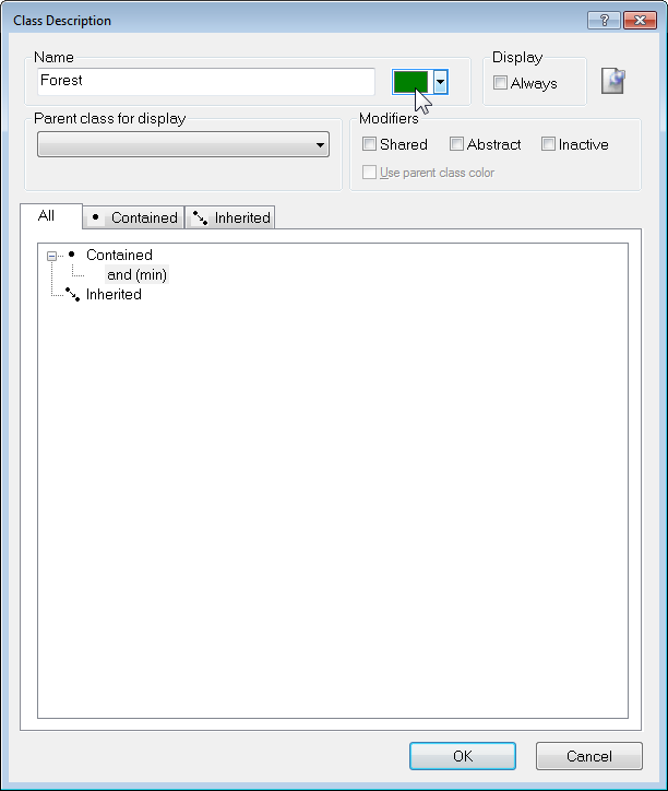
Enter a name for your class in the Name field and change the default color that is chosen randomly. (Default name: class. The second class inserted in the Class Hierarchy window obtains the default name class 1. Each time a new class is added the number is incremented by one.)
Press OK and your new class is listed in the Class Hierarchy window.
Creating a Class as Part of a Process
Many algorithms allow the creation of a new class. When the Class Filter parameter is listed under Parameters, clicking on the value will display the Edit Classification Filter dialog box. You can then right-click on this window, select Insert Class, then create a new class using the same method outlined in the preceding section.
The Assign Class Algorithm
The Assign Class algorithm is a simple classification algorithm, which allows you to assign a class based on a condition (for example a brightness range):
- Select Assign Class from the algorithm list in the Edit Process dialog box
- Edit the condition and define a condition that contains a feature (field Value 1) the desired comparison operator (field Operator), and a feature value (field Value 2).
In the Algorithm Parameters pane, opposite Use Class, select a class you have previously created, or enter a new name to create a new one (this will launch the Class Description dialog box)
Editing the Class Description
You can edit the class description to handle the features describing a certain class and the logic by which these features are combined.
- Open a class by double-clicking it in the Class Hierarchy window.
- To edit the class description, open either the All or the Contained tab.
- Insert or edit the expression to describe the requirements an image object must meet to be member of this class.
Inserting an Expression
A new or an empty class description contains the 'and (min)' operator by default.
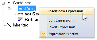
- To insert an expression, right-click the operator in the Class Description dialog and select Insert New Expression. Alternatively, double-click on the operator
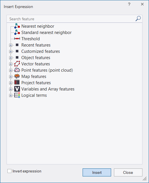
The Insert Expression dialog box opens, displaying all available features. - Navigate through the hierarchy to find a feature of interest
- Right-click the selected feature it to list more options:
- Insert Threshold: In the Edit Condition dialog box, set a condition for the selected feature, for example Area <= 100. Click OK to add the condition to the class description, then close the dialog box
- Insert Membership Function: In the Membership Function dialog box, edit the settings for the selected feature.
Although logical terms (operators) and similarities can be inserted into a class as they are, the nearest neighbor and the membership functions require further definition.
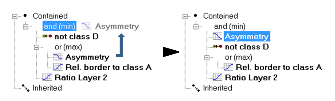
Moving an Expression
To move an expression, drag it to the desired location.
Editing an Expression
To edit an expression, double-click the expression or right-click it and choose Edit Expression from the context menu. Depending on the type of expression, one of the following dialog boxes opens:
- Edit Condition: Modifies the condition for a feature
- Membership Function: Modifies the membership function for a feature
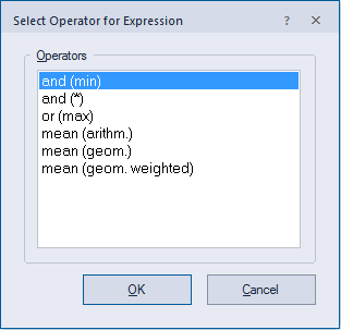
- Select Operator for Expression: Allows you to choose a logical operator from the list (see below)
- Edit Standard Nearest Neighbor Feature Space: Selects or deselects features for the standard nearest neighbor feature space
- Edit Nearest Neighbor Feature Space: Selects or deselects features for the nearest neighbor feature space.
Operator for Expression
The following expression operators are available in eCognition if you select Edit Expression or Insert expression > Logical terms:
- and (min) - 'and'-operator using the minimum function (default).
- and (*) - Product of feature values.
- or (max) - Fuzzy logical 'or'-operator using the maximum function.
- mean (arithm.) - Arithmetic mean of the assignment values (based on sum of values).
- mean (geom.) - Geometric mean of the assignment values (based on product of values).
- mean (geom. weighted) - Weighted geometric mean of the assignment values.
Example: Consider four membership values of 1 each and one of 0. The 'and'-operator yields the minimum value, i.e., 0, whereas the 'or'-operator yields the maximum value, i.e., 1. The arithmetic mean yields the average value, in this case a membership value of 0.8.
See also Fuzzy Classification using Operators and Adding Weightings to Membership Functions.
Evaluating Undefined Image Objects
Image objects retain the status 'undefined' when they do not meet the criteria of a feature. If you want to use these image objects anyway, for example for further processing, you must put them in a defined state. The function Evaluate Undefined assigns the value 0 for a specified feature.
- In the Class Description dialog box, right-click an operator
- From the context menu, select Evaluate Undefined. The expression below this operator is now marked.
Deleting an Expression
To delete an expression, either:
- Select the expression and press the Del button on your keyboard
- Right-click the expression and choose Delete Expression from the context menu.
Using Samples for Nearest Neighbor Classification
The Nearest Neighbor classifier is recommended when you need to make use of a complex combination of object features, or your image analysis approach has to follow a set of defined sample image objects. The principle is simple – first, the software needs samples that are typical representatives for each class. Based on these samples, the algorithm searches for the closest sample image object in the feature space of each image object. If an image object's closest sample object belongs to a certain class, the image object will be assigned to it.
For advanced users, the Feature Space Optimization function offers a method to mathematically calculate the best combination of features in the feature space. To classify image objects using the Nearest Neighbor classifier, follow the recommended workflow:
- Load or create classes
- Define the feature space
- Define sample image objects
- Classify, review the results and optimize your classification.
Defining Sample Image Objects For the Nearest Neighbor classification, you need sample image objects. These are image objects that you consider a significant representative of a certain class and feature. By doing this, you train the Nearest Neighbor classification algorithm to differentiate between classes. The more samples you select, the more consistent the classification. You can define a sample image object manually by clicking an image object in the map view.
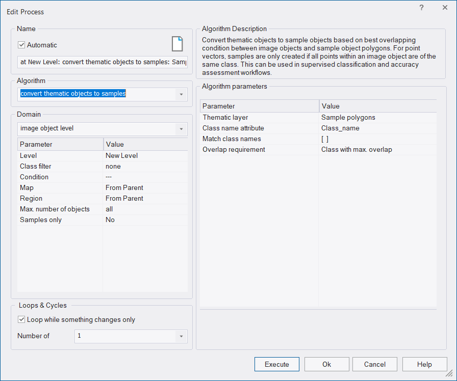
You can also add existing sample data in point or polygon vector layer format (e.g. using File > Add Data Layer...) and use it in a nearest neighbor classification based on the algorithm convert thematic objects to samples.
Adding Comments to an Expression
Comments can be added to expressions using the same principle described in Adding Comments to Classes.
The Edit Classification Filter
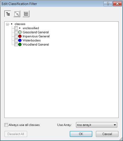
The Edit Classification Filter is available from the Edit Process dialog for appropriate algorithms (e.g. Algorithm classification) and can be launched from the Class Filter parameter.
The buttons at the top of the dialog allow you to:
- Select classes based on groups
- Select classes based on inheritance
- Select classes from a list (this option has a find function)
The Use Array drop-down box lets you filter classes based on arrays.
Classification Algorithms
The Assign Class Algorithm 
The Assign Class algorithm is the most simple classification algorithm. It uses a condition to determine whether an image object belongs to a class or not.
- In the Edit Process dialog box, select Assign Class from the Algorithm list
- The Image Object Level domain is selected by default. In the Parameter pane, select the Condition you wish to use and define the operator and reference value
- In the Class Filter, select or create a class to which the algorithm applies.
The Classification Algorithm 
The Classification algorithm uses class descriptions to classify image objects. It evaluates the class description and determines whether an image object can be a member of a class.
Classes without a class description are assumed to have a membership value of one. You can use this algorithm if you want to apply fuzzy logic to membership functions, or if you have combined conditions in a class description.
Based on the calculated membership value, information about the three best-fitting classes is stored in the image object classification window; therefore, you can see into what other classes this image object would fit and possibly fine-tune your settings. To apply this function:
- In the Edit Process dialog box, select classification from the Algorithm list and define the domain
- From the algorithm parameters, select active classes that can be assigned to the image objects
- Select Erase Old Classification to remove existing classifications that do not match the class description
- Select Use Class Description if you want to use the class description for classification. Class descriptions are evaluated for all classes. An image object is assigned to the class with the highest membership value.
The Hierarchical Classification Algorithm 
The Hierarchical Classification algorithm is used to apply complex class hierarchies to image object levels. It is backwards compatible with eCognition 4 and older class hierarchies and can open them without major changes.
The algorithm can be applied to an entire set of hierarchically arranged classes. It applies a predefined logic to activate and deactivate classes based on the following rules:
- Classes are not applied to the classification of image objects whenever they contain applicable child classes within the inheritance hierarchy.
Parent classes pass on their class descriptions to their child classes. (Unlike the Classification algorithm, classes without a class description are assumed to have a membership value of 0. )
These child classes then add additional feature descriptions and – if they are not parent classes themselves – are meaningfully applied to the classification of image objects. The above logic is following the concept that child classes are used to further divide a more general class. Therefore, when defining subclasses for one class, always keep in mind that not all image objects defined by the parent class are automatically defined by the subclasses. If there are objects that would be assigned to the parent class but none of the descriptions of the subclasses fit those image objects, they will be assigned to neither the parent nor the child classes. - Classes are only applied to a classification of image objects, if all contained classifiers are applicable.
The second rule applies mainly to classes containing class-related features. The reason for this is that you might generate a class that describes objects of a certain spectral value in addition to certain contextual information given by a class-related feature. The spectral value taken by itself without considering the context would cover far too many image objects, so that only a combination of the two would lead to satisfying results. As a consequence, when classifying without class-related features, not only the expression referring to another class but the whole class is not used in this classification process.
Contained and inherited expressions in the class description produce membership values for each object and according to the highest membership value, each object is then classified.
If the membership value of an image object is lower than the pre-defined minimum membership value, the image object remains unclassified. If two or more class descriptions share the highest membership value, the assignment of an object to one of these classes is random.
The three best classes are stored as the image object classification result. Class-related features are considered only if explicitly enabled by the corresponding parameter.
Using Hierarchical Classification with a Process
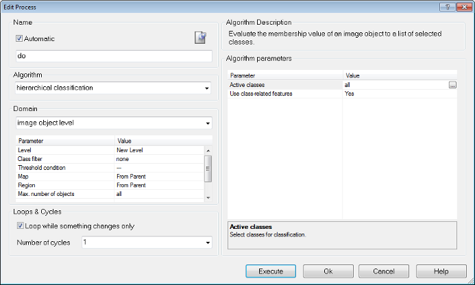
- In the Edit Process dialog box, select Hierarchical Classification from the Algorithm drop-down list
- Define the Domain if necessary.
- For the Algorithm Parameters, select the active classes that can be assigned to the image objects
- Select Use Class-Related Features if necessary.
Advanced Classification Algorithms
Advanced classification algorithms are designed to perform specific classification tasks. All advanced classification settings allow you to define the same classification settings as the classification algorithm; in addition, algorithm-specific settings must be set. The following algorithms are available:
- Find domain extrema allows identifying areas that fulfill a maximum or minimum condition within the defined domain
- Find local extrema allows identifying areas that fulfill a local maximum or minimum condition within the defined domain and within a defined search range around the object
- Find enclosed by class finds objects that are completely enclosed by a certain class
- Find enclosed by object finds objects that are completely enclosed by an image object
- Connector classifies image objects that represent the shortest connection between objects of a defined class.
Thresholds
Using Thresholds with Class Descriptions
A threshold condition determines whether an image object matches a condition or not. Typically, you use thresholds in class descriptions if classes can be clearly separated by a feature.
It is possible to assign image objects to a class based on only one condition; however, the advantage of using class descriptions lies in combining several conditions. The concept of threshold conditions is also available for process-based classification; in this case, the threshold condition is part of the domain and can be added to most algorithms. This limits the execution of the respective algorithm to only those objects that fulfill this condition. To use a threshold:
- Go to the Class Hierarchy dialog box and double-click on a class. Open the Contained tab of the Class Description dialog box. In the Contained area, right-click the initial operator 'and(min)' and choose Insert New Expression on the context menu
- From the Insert Expression dialog box, select the desired feature. Right-click on it and choose Insert Threshold from the context menu. The Edit Condition dialog box opens, where you can define the threshold expression
- In the Feature group box, the feature that has been selected to define the threshold is displayed on the large button at the top of the box. To select a different feature, click this button to reopen the Select Single Feature dialog box. Select a logical operator
- Enter the number defining the threshold; you can also select a variable if one exists. For some features such as constants, you can define the unit to be used and the feature range displays below it. Click OK to apply your settings. The resulting logical expression is displayed in the Class Description box.
About the Class Description
The class description contains class definitions such as name and color, along with several other settings. In addition it can hold expressions that describe the requirements an image object must meet to be a member of this class when class description-based classification is used. There are two types of expressions:
- Threshold expressions define whether a feature is fulfills a condition or not; for example whether it has a value of 1 or 0
- Membership functions apply fuzzy logic to a class description. You can define the degree of membership, for example any value between 1 (true) and 0 (not true). There are also several predefined types of membership functions that you can adapt:
- Use Samples for Nearest Neighbor Classification – this method lets you declare image objects to be significant members of a certain class. The Nearest Neighbor algorithm then finds image objects that resemble the samples
- Similarities allow you to use class descriptions of other classes to define a class. Similarities are most often expressed as inverted expressions.
You can use logical operators to combine the expressions and these expressions can be nested to produce complex logical expressions.
Using Membership Functions for Classification
Membership functions allow you to define the relationship between feature values and the degree of membership to a class using fuzzy logic.
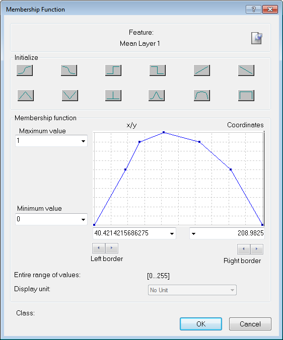
Double-clicking on a class in the Class Hierarchy window launches the Class Description dialog box. To open the Membership Function dialog, right-click on an expression – the default expression in an empty box is 'and (min)' – to insert a new one, select Insert New Expression. You can edit an existing one by right-clicking and selecting Edit Expression.
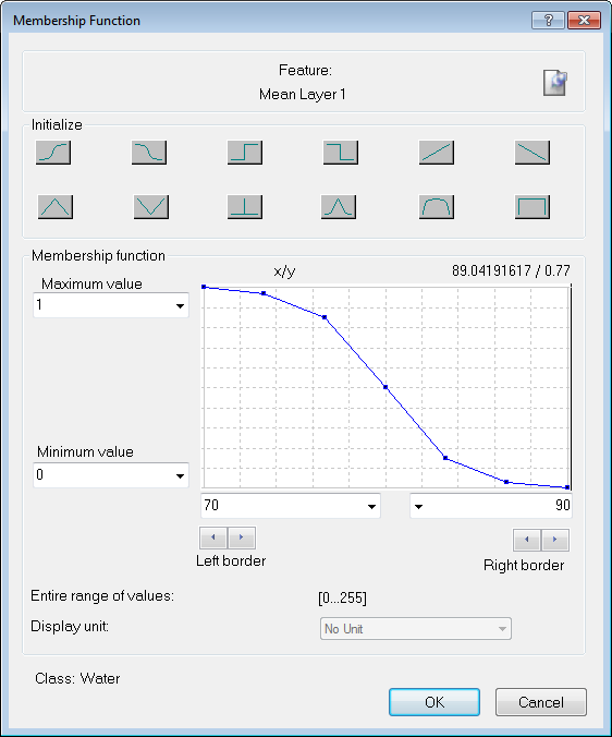
- The selected feature is displayed at the top of the box, alongside an icon that allows you to insert a comment
- The Initialize area contains predefined functions; these are listed in the next section. It is possible to drag points on the graph to edit the curve, although this is usually not necessary – we recommend you use membership functions that are as broad as possible
- Maximum Value and Minimum Value allow you to set the upper and lower limits of the membership function. (It is also possible to use variables as limits.)
- Left Border and Right Border values allow you to set the upper and lower limits of a feature value. In this example, the fuzzy value is between 100 and 1,000, so anything below 100 has a membership value of zero and anything above 1,000 has a membership value of one
- Entire Range of Values displays the possible value range for the selected feature
- For certain features you can edit the Display Unit
- The name of the class you are currently editing is displayed at the bottom of the dialog box.
- To display the comparable graphical output, go to the View Settings window and select Mode > Classification Membership.
Membership Function Type
For assigning membership, the following predefined functions are available:
| Button | Function Form |
|---|---|

|
Larger than |

|
Smaller than |

|
Larger than (Boolean, crisp) |

|
Smaller than (Boolean, crisp) |

|
Larger than (linear) |

|
Smaller than (linear) |

|
Linear range (triangle) |

|
Linear range (triangle inverted) |

|
Singleton (exactly one value) |

|
Approximate Gaussian |

|
About range |

|
Full range |
Fuzzy Classification using Operators
After the manual or automatic definition of membership functions, fuzzy logic can be applied to combine these fuzzified features with operators. Generally, fuzzy rules set certain conditions which result in a membership value to a class. If the condition only depends on one feature, no logic operators would be necessary to model it. However, there are usually multidimensional dependencies in the feature space and you may have to model a logic combination of features to represent this condition. This combination is performed with fuzzy logic. Fuzzy logic allows the modelling several concepts of 'and' and 'or'.
The most common and simplest combination is the realization of 'and' by the minimum operator and 'or' by the maximum operator. When the maximum operator 'or (max)' is used, the membership of the output equals the maximum fulfilment of the single statements. The maximum operator corresponds to the minimum operator 'and (min)' which equals the minimum fulfilment of the single statements. This means that out of a number of conditions combined by the maximum operator, the highest membership value is returned. If the minimum operator is used, the condition that produces the lowest value determines the return value. The other operators have the main difference that the values of all contained conditions contribute to the output, whereas for minimum and maximum only one statement determines the output.
When creating a new class, its conditions are combined with the minimum operator 'and (min)' by default. The default operator can be changed and additional operators can be inserted to build complex class descriptions, if necessary. For given input values the membership degree of the condition and therefore of the output will decrease with the following sequence:
- or (max): 'or'-operator returning the maximum of the fuzzy values, the strongest 'or'
- mean (arithm.): arithmetic mean of the fuzzy values
- and (min): 'and'-operator returning the minimum of the fuzzy values (used by default, the most reluctant 'and')
- mean (geom.): geometric mean of the fuzzy values / mean (geom. weighted): weighted geometric mean of the fuzzy values
- and (*): 'and'-operator returning the product of the fuzzy values
- Applicable to all operators above: not inversion of a fuzzy value: returns 1 – fuzzy value
See also Operator for Expression.
To change the default operator, right-click the operator and select 'Edit Expression.'
You can now choose from the available operators. To insert additional operators, open the 'Insert Expression' menu and select an operator under 'Logical Terms.' To insert an inverted operator, activate the 'Invert Expression' box in the same dialog; this negates the operator (returns 1 – fuzzy value): 'not and (min).' To combine classes with the newly inserted operators, click and drag the respective classes onto the operator.
A hierarchy of logical operator expressions can be combined to form well-structured class descriptions. Thereby, class descriptions can be designed very flexibly on the one hand, and very specifically on the other. An operator can combine either expressions only, or expressions and additional operators - again linking expressions.
An example of the flexibility of the operators is given in the image below. Both constellations represent the same conditions to be met in order to classify an object.
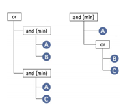
Generating Membership Functions Automatically
In some cases, especially when classes can be clearly distinguished, it is convenient to automatically generate membership functions. This can be done within the Sample Editor window (for more details on this function, see Working with the Sample Editor).
To generate a membership function, right-click the respective feature in the Sample Editor window and select Membership Functions > Compute.
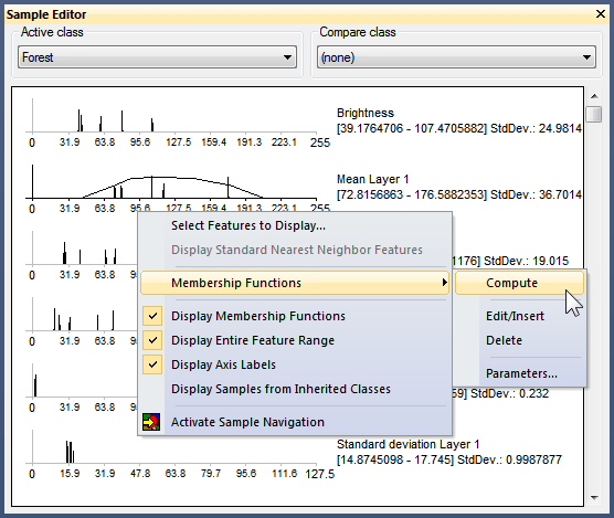
Membership functions can also be inserted and defined manually in the Sample Editor window. To do this, right-click a feature and select Membership Functions > Edit/Insert, which opens the Membership Function dialog box. This also allows you to edit an automatically generated function.
To delete a generated membership function, select Membership Functions > Delete. You can switch the display of generated membership functions on or off by right-clicking in the Sample Editor window and activating or deactivating Display Membership Functions.
Editing Membership Function Parameters
You can edit parameters of a membership function computed from sample objects.
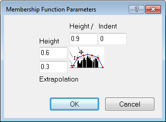
- In the Sample Editor, select Membership Functions > Parameters from the context menu. The Membership Function Parameters dialog box opens
- Edit the absolute Height of the membership function
- Modify the Indent of membership function
- Choose the Height of the linear part of the membership function
- Edit the Extrapolation width of the membership function.
Editing the Minimum Membership Value
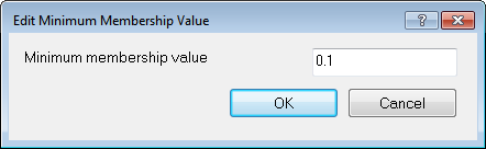
The minimum membership value defines the value an image object must reach to be considered a member of the class.
If the membership value of an image object is lower than a predefined minimum, the image object remains unclassified. If two or more class descriptions share the highest membership value, the assignment of an object to one of these classes is random.
To change the default value of 0.1, open the Edit Minimum Membership Value dialog box by selecting Classification > Advanced Settings > Edit Minimum Membership Value from the main menu.
Adding Weightings to Membership Functions
The following expressions support weighting:
- Mean (arithm.)
- Mean (geom.)
- Mean (geom. weighted)
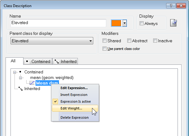
Weighting can be added to any expression by right-clicking on it and selecting Edit Weight. The weighting can be a positive number, or a scene or object variable. Information on weighting is also displayed in the Class Evaluation tab in the Object Information window.
Weights are integrated into the class evaluation value using the following formulas (where w = weight and m = membership value):
- Mean (arithm.)

- Mean (geom. weighted)

Using Similarities for Classification
Similarities work like the inheritance of class descriptions. Basically, adding a similarity to a class description is equivalent to inheriting from this class. However, since similarities are part of the class description, they can be used with much more flexibility than an inherited feature. This is particularly obvious when they are combined by logical terms.
A very useful method is the application of inverted similarities as a sort of negative inheritance: consider a class 'bright' if it is defined by high layer mean values. You can define a class 'dark' by inserting a similarity feature to bright and inverting it, thus yielding the meaning dark is not bright.
It is important to notice that this formulation of 'dark is not bright' refers to similarities and not to classification. An object with a membership value of 0.25 to the class 'bright' would be correctly classified as' bright'. If in the next cycle a new class dark is added containing an inverted similarity to bright the same object would be classified as 'dark', since the inverted similarity produces a membership value of 0.75. If you want to specify that 'dark' is everything which is not classified as 'bright' you should use the feature Classified As.
Similarities are inserted into the class description like any other expression.
Evaluation Classes
The combination of fuzzy logic and class descriptions is a powerful classification tool. However, it has some major drawbacks:
- Internal class descriptions are not the most transparent way to classify objects
- It does not allow you to use a given class several times in a variety of ways
- Changing a class description after a classification step deletes the original class description
- Classification will always occur when the Class Evaluation Value is greater than 0 (only one active class)
- Classification will always occur according to the highest Class Evaluation Value (several active classes)
There are two ways to avoid these problems – stagger several process containing the required conditions using the Parent Process Object concept (PPO) or use evaluation classes. Evaluation classes are as crucial for efficient development of auto-adaptive rule sets as variables and temporary classes.
Creating Evaluation Classes
To clarify, evaluation classes are not a specific feature and are created in exactly the same way as 'normal' classes. The idea is that evaluation classes will not appear in the classification result – they are better considered as customized features than real classes.
Like temporary classes, we suggest you prefix their names with '_Eval' and label them all with the same color, to distinguish them from other classes.
To optimize the thresholds for evaluation classes, click on the Class Evaluation tab in the Object Information window. Clicking on an object returns all of its defined values, allowing you to adjust them as necessary.
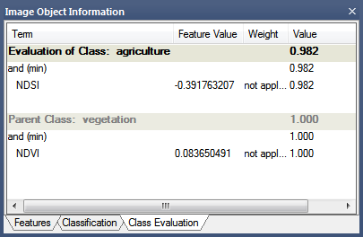
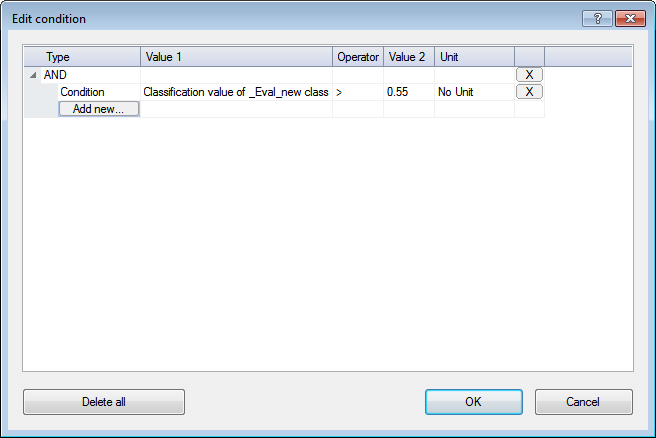
Using Evaluation Classes
In this example, the rule set developer has specified a threshold of 0.55. Rather than use this value in every rule set item, new processes simply refer to this evaluation class when entering a value for a threshold condition; if developers wish to change this value, they need only change the evaluation class.
TIP: When using this feature with the geometrical mean logical operator, ensure that no classifications return a value of zero, as the multiplication of values will also result in zero. If you want to return values between 0 and 1, use the arithmetic mean operator.
Supervised Classification
Video - Supervised classification - how to apply a supervised classification
Nearest Neighbor Classification
Classification with membership functions is based on user-defined functions of object features, whereas Nearest Neighbor classification uses a set of samples of different classes to assign membership values. The procedure consists of two major steps:
- Training the system by giving it certain image objects as samples
- Classifying image objects in the image object domain based on their nearest sample neighbors.
For a first introduction including a basic segmentation and simple supervised classification approach and export of the results - Video - Supervised Classification approach
The nearest neighbor classifies image objects in a given feature space and with given samples for the classes of concern. First the software needs samples, typical representatives for each class. After a representative set of sample objects has been declared the algorithm searches for the closest sample object in the defined feature space for each image object. The user can select the features to be considered for the feature space. If an image object's closest sample object belongs to Class A, the object will be assigned to Class A.
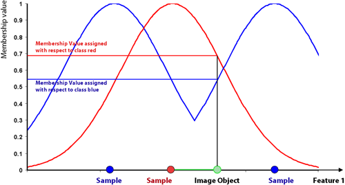
All class assignments in eCognition are determined by assignment values in the range 0 (no assignment) to 1 (full assignment). The closer an image object is located in the feature space to a sample of class A, the higher the membership degree to this class. The membership value has a value of 1 if the image object is identical to a sample. If the image object differs from the sample, the feature space distance has a fuzzy dependency on the feature space distance to the nearest sample of a class (see also Setting the Function Slope and Details on Calculation).
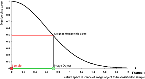
For an image object to be classified, only the nearest sample is used to evaluate its membership value. The effective membership function at each point in the feature space is a combination of fuzzy function over all the samples of that class. When the membership function is described as one-dimensional, this means it is related to one feature.
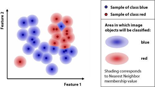
In higher dimensions, depending on the number of features considered, it is harder to depict the membership functions. However, if you consider two features and two classes only, it might look like the following graph:
Detailed Description of the Nearest Neighbor Calculation
eCognition computes the distance d as follows:


|
Distance between sample object s and image object o |

|
Feature value of sample object for feature f |

|
Feature value of image object for feature f |

|
Standard deviation of the feature values for feature f |
The distance in the feature space between a sample object and the image object to be classified is standardized by the standard deviation of all feature values. Thus, features of varying range can be combined in the feature space for classification. Due to the standardization, a distance value of d = 1 means that the distance equals the standard deviation of all feature values of the features defining the feature space.
Based on the distance d a multidimensional, exponential membership function z(d) is computed:

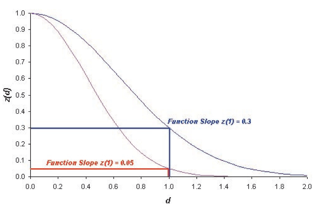
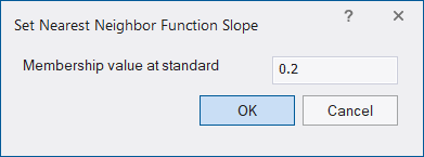
The parameter k determines the decrease of z(d). You can define this parameter with the variable function slope:

The default value for the function slope is 0.2. The smaller the parameter function slope, the narrower the membership function. Image objects have to be closer to sample objects in the feature space to be classified. If the membership value is less than the minimum membership value (default setting 0.1), then the image object is not classified. The following figure demonstrates how the exponential function changes with different function slopes.
Defining the Feature Space with Nearest Neighbor Expressions
To define feature spaces, Nearest Neighbor (NN) expressions are used and later applied to classes. eCognition Developer distinguishes between two types of nearest neighbor expressions:
- Standard Nearest Neighbor, where the feature space is valid for all classes it is assigned to within the project.
- Nearest Neighbor, where the feature space can be defined separately for each class by editing the class description.
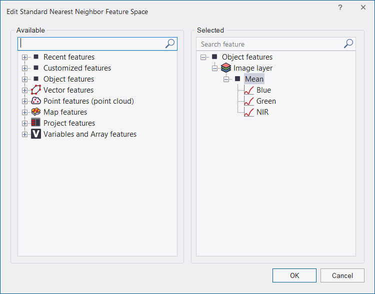
- From the main menu, choose Classification > Nearest Neighbor > Edit Standard NN Feature Space. The Edit Standard Nearest Neighbor Feature Space dialog box opens
- Double-click an available feature to send it to the Selected pane. (Class-related features only become available after an initial classification.)
- To remove a feature, double-click it in the Selected pane
- Use feature space optimization to combine the best features.
Applying the Standard Nearest Neighbor Classifier
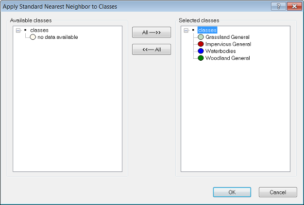
- From the main menu, select Classification > Nearest Neighbor > Apply Standard NN to Classes. The Apply Standard NN to Classes dialog box opens
- From the Available classes list on the left, select the appropriate classes by clicking on them
- To remove a selected class, click it in the Selected classes list. The class is moved to the Available classes list
- Click the All → button to transfer all classes from Available classes to Selected classes. To remove all classes from the Selected classes list, click the ← All button
- Click OK to confirm your selection
- In the Class Hierarchy window, double-click one class after the other to open the Class Description dialog box and to confirm that the class contains the Standard Nearest Neighbor expression.
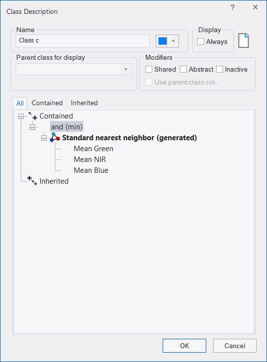
The Standard Nearest Neighbor feature space is now defined for the entire project. If you change the feature space in one class description, all classes that contain the Standard Nearest Neighbor expression are affected.
The feature space for both the Nearest Neighbor and the Standard Nearest Neighbor classifier can be edited by double-clicking them in the Class Description dialog box.
Once the Nearest Neighbor classifier has been assigned to all classes, the next step is to collect samples representative of each one.
Interactive Workflow for Nearest Neighbor Classification
Successful Nearest Neighbor classification usually requires several rounds of sample selection and classification. It is most effective to classify a small number of samples and then select samples that have been wrongly classified. Within the feature space, misclassified image objects are usually located near the borders of the general area of this class. Those image objects are the most valuable in accurately describing the feature space region covered by the class. To summarize:
- Insert Standard Nearest Neighbor into the class descriptions of classes to be considered
- Select samples for each class; initially only one or two per class
- Run the classification process. If image objects are misclassified, select more samples out of those and go back to step 2.
Optimizing the Feature Space
Feature Space Optimization is an instrument to help you find the combination of features most suitable for separating classes, in conjunction with a nearest neighbor classifier.
It compares the features of selected classes to find the combination of features that produces the largest average minimum distance between the samples of the different classes.
Using Feature Space Optimization
The Feature Space Optimization dialog box helps you optimize the feature space of a nearest neighbor expression.
To open the Feature Space Optimization dialog box, choose Tools > Feature Space Optimization or Classification > Nearest Neighbor > Feature Space Optimization from the main menu.
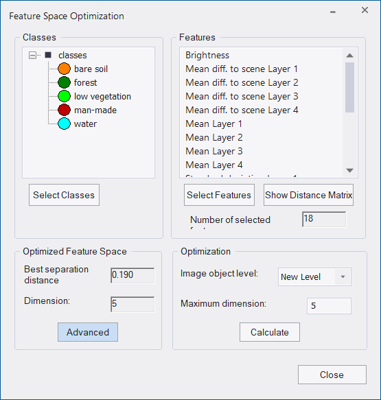
- To calculate the optimal feature space, press Select Classes to select the classes you want to calculate. Only classes for which you selected sample image objects are available for selection
- Click the Select Features button and select an initial set of features, which will later be reduced to the optimal number of features. You cannot use class-related features in the feature space optimization
- Highlight single features to select a subset of the initial feature space
- Select the image object level for the optimization
- Enter the maximum number of features within each combination. A high number reduces the speed of calculation
- Click Calculate to generate feature combinations and their distance matrices. (The distance calculation is only based upon samples. Therefore, adding or deleting samples also affects the separability of classes.)
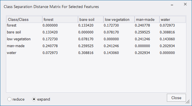
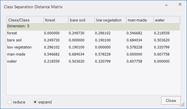
- Click Show Distance Matrix to display the Class Separation Distance Matrix for Selected Features dialog box. The matrix is only available after a calculation.
- The Best Separation Distance between the samples. This value is the minimum overall class combinations, because the overall separation is only as good as the separation of the closest pair of classes.
- After calculation, the Optimized Feature Space group box displays the following results:
- The Dimension indicates the number of features of the best feature combination.
- Click Advanced to open the Feature Space Optimization – Advanced Information dialog box and see more details about the results.
TIP: When you change any setting of features or classes, you must first click Calculate before the matrix reflects these changes.
Viewing Advanced Information
The Feature Space Optimization `– Advanced Information dialog box provides further information about all feature combinations and the separability of the class samples.
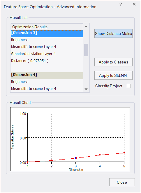
- The Result List displays all feature combinations and their corresponding distance values for the closest samples of the classes. The feature space with the highest result is highlighted by default
- The Result Chart shows the calculated maximum distances of the closest samples along the dimensions of the feature spaces. The blue dot marks the currently selected feature space
- Click the Show Distance Matrix button to display the Class Separation Distance Matrix window. This matrix shows the distances between samples of the selected classes within a selected feature space. Select a feature combination and re-calculate the corresponding distance matrix.
Using the Optimization Results
You can automatically apply the results of your Feature Space Optimization efforts to the project.
- In the Feature Space Optimization Advanced Information dialog box, click Apply to Classes to generate a nearest neighbor classifier using the current feature space for selected classes.
- Click Apply to Std. NN. to use the currently selected feature space for the Standard Nearest Neighbor classifier.
- Check the Classify Project checkbox to automatically classify the project when choosing Apply to Std. NN. or Apply to Classes.
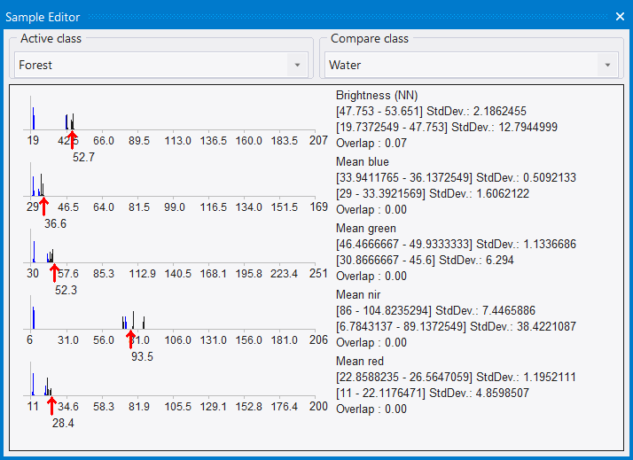
Working with the Sample Editor 
The Sample Editor window is the principal tool to input samples. For a selected class, it shows histograms of selected features of samples in the currently active map. The same values can be displayed for all image objects at a certain level or all levels in the image object hierarchy.
You can use the Sample Editor window to compare the attributes or histograms of image objects and samples of different classes. It is helpful to get an overview of the feature distribution of image objects or samples of specific classes. The features of an image object can be compared to the total distribution of this feature over one or all image object levels.
Use this tool to assign samples using a Nearest Neighbor classification or to compare an image object to already existing samples, in order to determine to which class an image object belongs. If you assign samples, features can also be compared to the samples of other classes. Only samples of the currently active map are displayed.
It is helpful to open the sample toolbar via View > Toolbars > Samples.
- Open the Sample Editor window using Classification > Samples > Sample Editor from the main menu.
- By default, the Sample Editor window shows diagrams for only a selection of features. To select the features to be displayed in the Sample Editor, right-click in the Sample Editor window and choose Select Features to Display.
- In the Select Displayed Features dialog box, double-click a feature from the left-hand pane to select it. To remove a feature, click it in the right-hand pane.
- To add the features used for the Standard Nearest Neighbor expression, select Display Standard Nearest Neighbor Features from the context menu.
Comparing Features
To compare samples or layer histograms of two classes, select the classes or the levels you want to compare in the Active Class and Compare Class lists.
Values of the active class are displayed in black in the diagram, the values of the compared class in blue. The value range and standard deviation of the samples are displayed on the right-hand side.
Viewing the Value of an Image Object
When you select an image object, the feature value is highlighted with a red pointer. This enables you to compare different objects with regard to their feature values. The following functions help you to work with the Sample Editor:
- The feature range displayed for each feature is limited to the currently detected feature range. To display the whole feature range, select Display Entire Feature Range from the context menu
- To hide the display of the axis labels, deselect Display Axis Labels from the context menu
- To display the feature value of samples from inherited classes, select Display Samples from Inherited Classes
- To navigate to a sample image object in the map view, click on the red arrow in the Sample Editor.
In addition, the Sample Editor window allows you to generate membership functions. The following options are available:
- To insert a membership function to a class description, select Display Membership Function > Compute from the context menu
- To display membership functions graphs in the histogram of a class, select Display Membership Functions from the context menu
- To insert a membership function or to edit an existing one for a feature, select the feature histogram and select Membership Function > Insert/Edit from the context menu
- To delete a membership function for a feature, select the feature histogram and select Membership Function > Delete from the context menu
- To edit the parameters of a membership function, select the feature histogram and select Membership Function > Parameters from the context menu.
Selecting Samples 
A Nearest Neighbor classification needs training areas. Therefore, representative samples of image objects need to be collected (or alternatively loaded as a thematic layer - see below About Classification).
- To assign sample objects, activate the input mode. Choose Classification > Samples > Select Samples from the main menu bar. The map view changes to the View Samples mode.
- To open the Sample Editor window, which helps to gather adequate sample image objects, do one of the following:
- Choose Classification > Samples > Sample Editor from the main menu.
- Choose View > Windows > Sample Editor from the main menu.
- To select a class from which you want to collect samples, do one of the following:
- Select the class in the Class Hierarchy window if available.
- Select the class from the Active Class drop-down list in the Sample Editor window.
This makes the selected class your active class so any samples you collect will be assigned to that class.
- To define an image object as a sample for a selected class, double-click the image object in the map view. To undo the declaration of an object as sample, double-click it again. You can select or deselect multiple objects by holding down the Shift key.
As long as the sample input mode is activated, the view will always change back to the Sample View when an image object is selected. Sample View displays sample image objects in the class color; this way the accidental input of samples can be avoided. - To view the feature values of the sample image object, go to the Sample Editor window. This enables you to compare different image objects with regard to their feature values.
- Click another potential sample image object for the selected class. Analyze its membership value and its membership distance to the selected class and to all other classes within the feature space. Here you have the following options:
- The potential sample image object includes new information to describe the selected class: low membership value to selected class, low membership value to other classes.
- The potential sample image object is really a sample of another class: low membership value to selected class, high membership value to other classes.
- The potential sample image object is needed as sample to distinguish the selected class from other classes: high membership value to selected class, high membership value to other classes.
In the first iteration of selecting samples, start with only a few samples for each class, covering the typical range of the class in the feature space. Otherwise, its heterogeneous character will not be fully considered.
- Repeat the same for remaining classes of interest.
- Classify the scene.
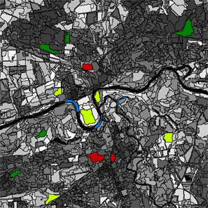
- The results of the classification are now displayed in the map view. In the View Settings dialog box, the mode has changed from Samples to Classification.
- Note that some image objects may have been classified incorrectly or not at all. All image objects that are classified are displayed in the appropriate class color. If you hover the cursor over a classified image object, a tool -tip pops up indicating the class to which the image object belongs, its membership value, and whether or not it is a sample image object. Image objects that are unclassified appear transparent. If you hover over an unclassified object, a tool-tip indicates that no classification has been applied to this image object. This information is also available in the Classification tab of the Information window.
- The refinement of the classification result is an iterative process:
- First, assess the quality of your selected samples
- Then, remove samples that do not represent the selected class well and add samples that are a better match or have previously been misclassified
- Classify the scene again
- Repeat this step until you are satisfied with your classification result.
- When you have finished collecting samples, remember to turn off the Select Samples input mode. (Note that the sample input mode is deactivated as soon as you change your view settings or close the sample toolbar and classification view is activated.)
Assessing the Quality of Samples
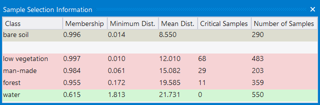
Once a class has at least one sample, the quality of a new sample can be assessed in the Sample Selection Information window. It can help you to decide if an image object contains new information for a class, or if it should belong to another class.
- To open the Sample Selection Information window choose Classification > Samples > Sample Selection Information or View > Toolbars > Samples > Sample Selection Information
- Names of classes are displayed in the Class column. The Membership column shows the membership value of the Nearest Neighbor classifier for the selected image object
- The Minimum Dist. column displays the distance in feature space to the closest sample of the respective class
- The Mean Dist. column indicates the average distance to all samples of the corresponding class
- The Critical Samples column displays the number of samples within a critical distance to the selected class in the feature space
- The Number of Samples column indicates the number of samples selected for the corresponding class.
The following highlight colors are used for a better visual overview:- Gray: Used for the selected class.
- Red: Used if a selected sample is critically close to samples of other classes in the feature space.
- Green: Used for all other classes that are not in a critical relation to the selected class.
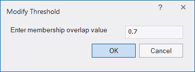
The critical sample membership value can be changed by right-clicking inside the window. Select Modify Critical Sample Membership Overlap from the context menu. The default value is 0.7, which means all membership values higher than 0.7 are critical.
To select which classes are shown, right-click inside the dialog box and choose Select Classes to Display.
Navigating Samples 
To navigate to samples in the map view, select samples in the Sample Editor window to highlight them in the map view.
- Before navigating to samples you must select a class in the Select Sample Information dialog box.
- To activate Sample Navigation , do one of the following:
- Choose Classification > Samples > Sample Editor Options > Activate Sample Navigation from the main menu
- Right-click inside the Sample Editor and choose Activate Sample Navigation from the context menu.
- To navigate samples, click in a histogram displayed in the Sample Editor window. A selected sample is highlighted in the map view and in the Sample Editor window.
- If there are two or more samples so close together that it is not possible to select them separately, you can use one of the following:
- Select a Navigate to Sample button.
- Select from the sample selection drop-down list.

Deleting Samples
- Deleting samples means to unmark sample image objects. They continue to exist as regular image objects.
- To delete a single sample, double-click or Shift-click it.
- To delete samples of specific classes, choose one of the following from the main menu:
- Classification > Class Hierarchy > Edit Classes > Delete Samples, which deletes all samples from the currently selected class.
- Classification > Samples > Delete Samples of Classes, which opens the Delete Samples of Selected Classes dialog box. Move the desired classes from the Available Classes to the Selected Classes list (or vice versa) and click OK
- To delete all samples you have assigned, select Classification > Samples > Delete All Samples.
Alternatively you can delete samples by using the Delete All Samples algorithm or the Delete Samples of Class algorithm.
Creating Samples based on a thematic Layer
You can use thematic layers to create sample image objects.
Using a thematic layer for sample creation comprises the following steps:
- If not loaded already - open a project and load the thematic layer into a map that contains sample information.
- Apply the algorithm 'convert thematic objects to samples' (see also Reference Book > Algorithms > Sample Operation Algorithms Convert thematic Objects to Samples )
- Classify image objects using the samples.
How to add a thematic layer to an existing project
- Open the project and select a map
- Select File > Modify Open Project from the main menu. The Modify Project dialog box opens.
- Insert the thematic layer as a new thematic layer. Confirm with OK.
Selecting Samples with the Sample Brush 
The Sample Brush is an interactive tool that allows you to use your cursor like a brush, creating samples as you sweep it across the map view. Go to the Sample Editor toolbar (View > Toolbars > Sample Editor) and press the Select Sample button. Right-click on the image in map view and select Sample Brush.
Drag the cursor across the scene to select samples. By default, samples are not reselected if the image objects are already classified but existing samples are replaced if drag over them again. These settings can be changed in the Sample Brush group of the Options dialog box. To deselect samples, press Shift as you drag.
The Sample Brush will select up to one hundred image objects at a time, so you may need to increase magnification if you have a large number of image objects.
Setting the Nearest Neighbor Function Slope
The Nearest Neighbor Function Slope defines the distance an object may have from the nearest sample in the feature space while still being classified. Enter values between 0 and 1. Higher values result in a larger number of classified objects.
- To set the function slope, choose Classification > Nearest Neighbor > Set NN Function Slope from the main menu bar.
- Enter a value and click OK.
Using Class-Related Features in a Nearest Neighbor Feature Space
To prevent non-deterministic classification results when using class-related features in a nearest neighbor feature space, several constraints have to be mentioned:
- It is not possible to use the feature Similarity To with a class that is described by a nearest neighbor with class-related features.
- Classes cannot inherit from classes that use nearest neighbor-containing class-related features. Only classes at the bottom level of the inheritance class hierarchy can use class-related features in a nearest neighbor.
- It is impossible to use class-related features that refer to classes in the same group including the group class itself.
Supervised Classification Algorithms (former name 'Classifier')
Overview
The supervised classification algorithm allows classifying based on different statistical classification algorithms:
- Bayes
- KNN (K Nearest Neighbor)
- SVM (Support Vector Machine)
- Decision Tree
- Random Trees
The algorithm can be applied either pixel- or object-based. For an examples project containing please refer to the eCognition Knowledge-Base and Tutorials.
Bayes
A Bayes classifier is a simple probabilistic classifier based on applying Bayes’ theorem (from Bayesian statistics) with strong independence assumptions. In simple terms, a Bayes classifier assumes that the presence (or absence) of a particular feature of a class is unrelated to the presence (or absence) of any other feature. For example, a fruit may be considered to be an apple if it is red, round, and about 4” in diameter. Even if these features depend on each other or upon the existence of the other features, a Bayes classifier considers all of these properties to independently contribute to the probability that this fruit is an apple. An advantage of the naive Bayes classifier is that it only requires a small amount of training data to estimate the parameters (means and variances of the variables) necessary for classification. Because independent variables are assumed, only the variances of the variables for each class need to be determined and not the entire covariance matrix.
KNN (K Nearest Neighbor)
The k-nearest neighbor algorithm (k-NN) is a method for classifying objects based on closest training examples in the feature space. k-NN is a type of instance-based learning, or lazy learning where the function is only approximated locally and all computation is deferred until classification. The k-nearest neighbor algorithm is amongst the simplest of all machine learning algorithms: an object is classified by a majority vote of its neighbors, with the object being assigned to the class most common amongst its k nearest neighbors (k is a positive integer, typically small). The 5-nearest-neighbor classification rule is to assign to a test sample the majority class label of its 5 nearest training samples. If k = 1, then the object is simply assigned to the class of its nearest neighbor.
This means k is the number of samples to be considered in the neighborhood of an unclassified object/pixel. The best choice of k depends on the data: larger values reduce the effect of noise in the classification, but the class boundaries are less distinct.
eCognition software has the Nearest Neighbor implemented as a classifier that can be applied using the algorithm classifier (KNN with k=1) or using the concept of classification based on the Nearest Neighbor Classification.
SVM (Support Vector Machine)
A support vector machine (SVM) is a concept in computer science for a set of related supervised learning methods that analyze data and recognize patterns, used for classification and regression analysis. The standard SVM takes a set of input data and predicts, for each given input, which of two possible classes the input is a member of. Given a set of training examples, each marked as belonging to one of two categories, an SVM training algorithm builds a model that assigns new examples into one category or the other. An SVM model is a representation of the examples as points in space, mapped so that the examples of the separate categories are pided by a clear gap that is as wide as possible. New examples are then mapped into that same space and predicted to belong to a category based on which side of the gap they fall on. Support Vector Machines are based on the concept of decision planes defining decision boundaries. A decision plane separates between a set of objects having different class memberships.
Important parameters for SVM
There are different kernels that can be used in Support Vector Machines models. Included in eCognition are linear and radial basis function (RBF). The RBF is the most popular choice of kernel types used in Support Vector Machines. Training of the SVM classifier involves the minimization of an error function with C as the capacity constant.
Decision Tree (CART resp. classification and regression tree)
Decision tree learning is a method commonly used in data mining where a series of decisions are made to segment the data into homogeneous subgroups. The model looks like a tree with branches - while the tree can be complex, involving a large number of splits and nodes. The goal is to create a model that predicts the value of a target variable based on several input variables. A tree can be “learned” by splitting the source set into subsets based on an attribute value test. This process is repeated on each derived subset in a recursive manner called recursive partitioning. The recursion is completed when the subset at a node all has the same value of the target variable, or when splitting no longer adds value to the predictions. The purpose of the analyses via tree-building algorithms is to determine a set of if-then logical (split) conditions.
Important Decision Tree parameters
The minimum number of samples that are needed per node are defined by the parameter Min sample count. Finding the right sized tree may require some experience. A tree with too few of splits misses out on improved predictive accuracy, while a tree with too many splits is unnecessarily complicated. Cross validation exists to combat this issue by setting eCognitions parameter Cross validation folds. For a cross-validation the classification tree is computed from the learning sample, and its predictive accuracy is tested by test samples. If the costs for the test sample exceed the costs for the learning sample this indicates poor cross-validation and that a different sized tree might cross-validate better.
Random Trees
The random trees classifier is more a framework that a specific model. It uses an input feature vector and classifies it with every tree in the forest. It results in a class label of the training sample in the terminal node where it ends up. This means the label is assigned that obtained the majority of "votes". Iterating this over all trees results in the random forest prediction. All trees are trained with the same features but on different training sets, which are generated from the original training set. This is done based on the bootstrap procedure: for each training set the same number of vectors as in the original set ( =N ) is selected. The vectors are chosen with replacement which means some vectors will appear more than once and some will be absent. At each node not all variables are used to find the best split but a randomly selected subset of them. For each node a new subset is construced, where its size is fixed for all the nodes and all the trees. It is a training parameter, set to  . None of the trees that are built are pruned.
In random trees the error is estimated internally during the training. When the training set for the current tree is drawn by sampling with replacement, some vectors are left out. This data is called out-of-bag data - in short "oob" data. The oob data size is about N/3. The classification error is estimated based on this oob-data.
Classification using the Sample Statistics Table
Overview
The supervised classification algorithm allows a classification based on sample statistics.
As described in the Reference Book > Advanced Classification Algorithms > Update supervised sample statistics and Export supervised sample statistics you can apply statistics generated with eCognition’s algorithms to classify your imagery.
Detailed Workflow
A typical workflow comprises the following steps:
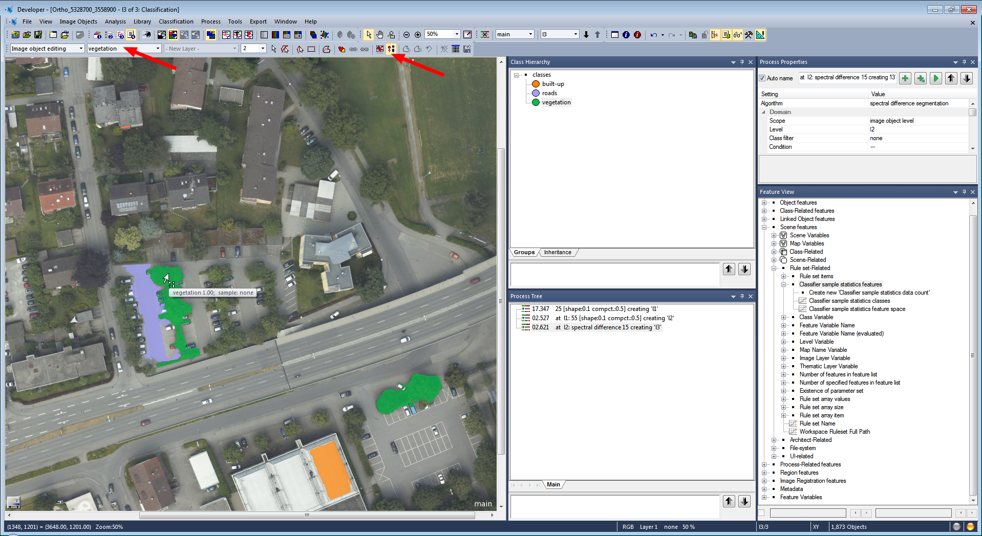
Input of Image Objects for Supervised Sample Statistics
- Create a new project and apply a segmentation
- Insert classes in the class hierarchy or load an existing class hierarchy
- Open View > Toolbars > Manual Editing Toolbar
- In the Image object editing mode select your classes (second drop-down menu) and classify image objects manually using the Classify Image Objects button.
Generate a Supervised Sample Statistics
- To understand what happens when executing the following algorithm you can visualize the following features in the Object Information dialog:
- Right-click in the dialog > Select Features to Display > Available > Project features > Samples > Supervised sample statistics features
- Double-click all features to switch them to the Selected side of this dialog (for the feature Create new 'Supervised sample statistics data count' keep the default settings and select OK).
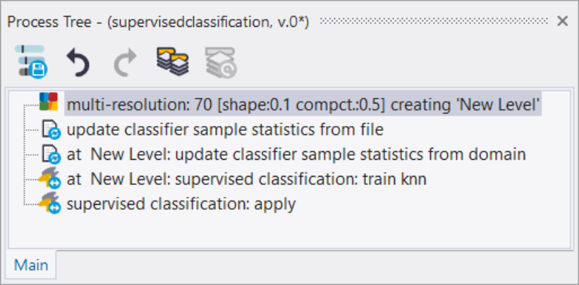
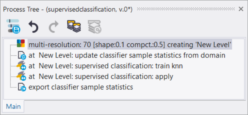
- Insert and execute the process update supervised sample statistics in the Process Tree Window with the following settings:
- Domain > image object level
- Parameter > Level: choose the appropriate level
- Parameter > Class filter: activate all classes
- Algorithm parameters > Parameter > Feature: select features to be applied in the statistics file (e.g. Mean Layer 1-3).
- The Object Information dialog shows you which classes are included in the sample statistics, how many sample objects are selected and which feature space is applied. Each time you execute the process update supervised sample statistics the contents are updated.
Classification using Sample Statistics
- Insert and execute the process supervised classification with the settings:
- Domain > image object level
- Parameter > Level: choose the appropriate level
- Algorithm parameters > Operation > Train (default)
- Algorithm parameters > Configuration: insert a string variable e.g. config1 > in the Create Scene Variable dialog change the value type from Double to String. (Variables can be changed also in the Menu Process > Manage Variables > Scene).
- Algorithm parameters > Feature Space > Source > select sample statistics based
- Algorithm parameters > Classifier > Type > select the classifier for your classification e.g. KNN
- Insert and execute the process supervised classificationagain with the settings:
- Domain > image object level
- Parameter > Level: choose the appropriate level
- Algorithm parameters > Operation > Apply
- Algorithm parameters > Configuration: select your configuration, e.g. config1
- Algorithm parameters > Feature Space > Source > select sample statistics based
Export a Supervised Sample Statistics Table
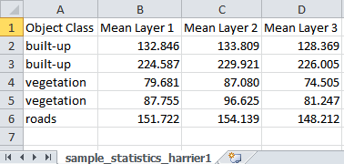
- Insert and execute the process export supervised sample statistics to export the samples statistics table e.g. Sample_Statistics1.csv
- Open the exported table and check the results - you can see for each sample the feature statistics.
Apply Sample Statistics Table to another Scene
- Create a new project/workspace with imagery to apply the sample statistics table. The project should be segmented already.
- Optional: To check whether features of the sample statistics project and the current project differ you can apply a validation using the process update supervised sample statistics in the Process Tree Window with the settings:
- Algorithm parameters > Mode > validate
- Algorithm parameters > Sample statistics file: browse to select the statistics table to be validated e.g. Sample_Statistics1.csv
- Algorithm parameters > Features not existing: insert name
- Algorithm parameters > Features not in classifier table: insert name
- Algorithm parameters > Features not in statistics file: insert name
- Insert and execute the process update supervised sample statistics in the Process Tree Window with the settings:
- Algorithm parameters > Mode > load
- Algorithm parameters > Sample statistics file: browse to select the statistics table to be validated e.g. Sample_Statistics1.csv
Classes from the sample statistics file are loaded to your project together with the sample statistics information.
-
You can now add more samples using the manual editing toolbar (same workflow as described in Input of Image Objects for Supervised Sample Statistics). These samples can be added in the following step to the loaded samples of the statistics file.
-
Insert the process update supervised sample statistics with the settings:
Domain > image object level
Parameter > Level: choose the appropriate level
- Parameter > Class filter: activate all classes
- Algorithm parameters > Parameter > Feature: select the same features as in the statistics file
Execute this process and have a look again at the features:
- Supervised sample statistics data count all : number of new inserted sample objects and loaded statistics table objects
- Supervised sample statistics data count external: samples loaded from the statistics table
- Supervised sample statistics data count local : inserted sample objects of the current project
Note: To reset samples you can execute the process update supervised sample statistics in mode:
- clear all: removes external loaded and local samples or
- clear local: removes only manual selected sample objects of the current project
-
- Insert and execute the process supervised classification with the settings:
- Domain > image object level
- Parameter > Level: choose the appropriate level
- Algorithm parameters > Operation > Train (default)
- Algorithm parameters > Configuration: insert a value e.g. config1 > in the Create Scene Variable dialog change the value type from Double to String.
- Algorithm parameters > Feature Space > Source > select sample statistics based
- Algorithm parameters > Classifier > Type > select the classifier for your classification e.g. KNN
- Insert and execute the process supervised classification again with the settings:
- Domain > image object level
- Parameter > Level: choose the appropriate level
- Algorithm parameters > Operation > Apply
- Algorithm parameters > Configuration: select your configuration, e.g. config1
- Algorithm parameters > Feature Space > Source > select sample statistics based
Now the image is classified and the described steps can be repeated based on another scene to refine the sample statistics iteratively.